102. Competitive Equilibria with Arrow Securities#
102.1. Introduction#
This lecture presents Python code for experimenting with competitive equilibria of an infinite-horizon pure exchange economy with
Heterogeneous agents
Endowments of a single consumption that are person-specific functions of a common Markov state
Complete markets in one-period Arrow state-contingent securities
Discounted expected utility preferences of a kind often used in macroeconomics and finance
Common expected utility preferences across agents
Common beliefs among agents
A constant relative risk aversion (CRRA) one-period utility function that implies the existence of a representative consumer whose consumption process can be plugged into a formula for the pricing kernel for one-step Arrow securities and thereby determine equilibrium prices before determining an equilibrium distribution of wealth
Differences in their endowments make individuals want to reallocate consumption goods across time and Markov states
We impose restrictions that allow us to Bellmanize competitive equilibrium prices and quantities
We use Bellman equations to describe
asset prices
continuation wealth levels for each person
state-by-state natural debt limits for each person
In the course of presenting the model we shall encounter these important ideas
a resolvent operator widely used in this class of models
absence of borrowing limits in finite horizon economies
state-by-state borrowing limits required in infinite horizon economies
a counterpart of the law of iterated expectations known as a law of iterated values
a state-variable degeneracy that prevails within a competitive equilibrium and that opens the way to various appearances of resolvent operators
102.2. The setting#
In effect, this lecture implements a Python version of the model presented in section 9.3.3 of Ljungqvist and Sargent [Ljungqvist and Sargent, 2018].
102.2.1. Preferences and endowments#
In each period \(t\geq 0\), a stochastic event \(s_t \in {\bf S}\) is realized.
Let the history of events up until time \(t\) be denoted \(s^t = [s_0, s_{1}, \ldots, s_{t-1}, s_t]\).
(Sometimes we inadvertently reverse the recording order and denote a history as \(s^t = [s_t, s_{t-1}, \ldots, s_1, s_0]\).)
The unconditional probability of observing a particular sequence of events \(s^t\) is given by a probability measure \(\pi_t(s^t)\).
For \(t > \tau\), we write the probability of observing \(s^t\) conditional on the realization of \(s^\tau\) as \(\pi_t(s^t\vert s^\tau)\).
We assume that trading occurs after observing \(s_0\), which we capture by setting \(\pi_0(s_0)=1\) for the initially given value of \(s_0\).
In this lecture we shall follow much macroeconomics and econometrics and assume that \(\pi_t(s^t)\) is induced by a Markov process.
There are \(K\) consumers named \(k=1, \ldots , K\).
Consumer \(k\) owns a stochastic endowment of one good \(y_t^k(s^t)\) that depends on the history \(s^t\).
The history \(s^t\) is publicly observable.
Consumer \(k\) purchases a history-dependent consumption plan \(c^k = \{c_t^k(s^t)\}_{t=0}^\infty\)
Consumer \(k\) orders consumption plans by
where \(0 < \beta < 1\).
The right side is equal to \( E_0 \sum_{t=0}^\infty \beta^t u_k(c_t^k) \), where \(E_0\) is the mathematical expectation operator, conditioned on \(s_0\).
Here \(u_k(c)\) is an increasing, twice continuously differentiable, strictly concave function of consumption \(c\geq 0\) of one good.
The utility function of person \(k\) satisfies the Inada condition
This condition implies that each agent chooses strictly positive consumption for every date-history pair \((t, s^t)\).
Those interior solutions enable us to confine our analysis to Euler equations that hold with equality and also guarantee that natural debt limits don’t bind in economies like ours with sequential trading of Arrow securities.
We adopt the assumption, routinely employed in much of macroeconomics, that consumers share probabilities \(\pi_t(s^t)\) for all \(t\) and \(s^t\).
A feasible allocation satisfies
for all \(t\) and for all \(s^t\).
102.3. Recursive formulation#
Following descriptions in section 9.3.3 of Ljungqvist and Sargent [Ljungqvist and Sargent, 2018] chapter 9, we set up a competitive equilibrium of a pure exchange economy with complete markets in one-period Arrow securities.
When endowments \(y^k(s)\) are all functions of a common Markov state \(s\), the pricing kernel takes the form \(Q(s'|s)\), where \(Q(s'| s)\) is the price of one unit of consumption in state \(s'\) at date \(t+1\) when the Markov state at date \(t\) is \(s\).
These enable us to provide a recursive formulation of a consumer’s optimization problem.
Consumer \(k\)’s state at time \(t\) is its financial wealth \(a^k_t\) and Markov state \(s_t\).
Let \(v^k(a,s)\) be the optimal value of consumer \(k\)’s problem starting from state \((a, s)\).
\(v^k(a,s)\) is the maximum expected discounted utility that consumer \(k\) with current financial wealth \(a\) can attain in Markov state \(s\).
The optimal value function satisfies the Bellman equation
where maximization is subject to the budget constraint
and also the constraints
with the second constraint evidently being a set of state-by-state debt limits.
Note that the value function and decision rule that solve the Bellman equation implicitly depend on the pricing kernel \(Q(\cdot \vert \cdot)\) because it appears in the agent’s budget constraint.
Use the first-order conditions for the problem on the right of the Bellman equation and a Benveniste-Scheinkman formula and rearrange to get
where it is understood that \(c_t^k = c^k(s_t)\) and \(c_{t+1}^k = c^k(s_{t+1})\).
Definition 102.1
A recursive competitive equilibrium is an initial distribution of wealth \(\vec a_0\), a set of borrowing limits \(\{\bar A^k(s)\}_{k=1}^K\), a pricing kernel \(Q(s' | s)\), sets of value functions \(\{v^k(a,s)\}_{k=1}^K\), and decision rules \(\{c^k(s), \hat a^k(s)\}_{k=1}^K\) such that
The state-by-state borrowing constraints satisfy the recursion
For all \(k\), given \(a^k_0\), \(\bar A^k(s)\), and the pricing kernel, the value functions and decision rules solve the consumers’ problems;
For all realizations of \(\{s_t\}_{t=0}^\infty\), the consumption and asset portfolios \(\{\{c^k_t,\) \(\{\hat a^k_{t+1}(s')\}_{s'}\}_k\}_t\) satisfy \(\sum_k c^k_t = \sum_k y^k(s_t)\) and \(\sum_k \hat a_{t+1}^k(s') = 0\) for all \(t\) and \(s'\).
The initial financial wealth vector \(\vec a_0\) satisfies \(\sum_{k=1}^K a_0^k = 0 \).
The third condition asserts that there are zero net aggregate claims in all Markov states.
The fourth condition asserts that the economy is closed and starts from a situation in which there are zero net aggregate claims.
102.4. State variable degeneracy#
Please see Ljungqvist and Sargent [Ljungqvist and Sargent, 2018] for a description of timing protocol for trades consistent with an Arrow-Debreu vision in which
at time \(0\) there are complete markets in a complete menu of history \(s^t\)-contingent claims on consumption at all dates that all trades occur at time zero
all trades occur once and for all at time \(0\)
If an allocation and pricing kernel \(Q\) in a recursive competitive equilibrium are to be consistent with the equilibrium allocation and price system that prevail in a corresponding complete markets economy with such history-contingent commodities and all trades occurring at time \(0\), we must impose that \(a_0^k = 0\) for \(k = 1, \ldots , K\).
That is what assures that at time \(0\) the present value of each agent’s consumption equals the present value of his endowment stream, the single budget constraint in arrangement with all trades occurring at time \(0\).
Starting the system with \(a_0^k =0\) for all \(i\) has a striking implication that we call state variable degeneracy.
Here is what we mean by state variable degeneracy:
Although two state variables \(a,s\) appear in the value function \(v^k(a,s)\), within a recursive competitive equilibrium starting from \(a_0^k = 0 \ \forall i\) at initial Markov state \(s_0\), two outcomes prevail:
\(a_0^k = 0 \) for all \(i\) whenever the Markov state \(s_t\) returns to \(s_0\).
Financial wealth \(a\) is an exact function of the Markov state \(s\).
The first finding asserts that each household recurrently visits the zero financial wealth state with which it began life.
The second finding asserts that within a competitive equilibrium the exogenous Markov state is all we require to track an individual.
Financial wealth turns out to be redundant because it is an exact function of the Markov state for each individual.
This outcome depends critically on there being complete markets in Arrow securities.
For example, it does not prevail in the incomplete markets setting of this lecture The Aiyagari Model
102.5. Markov asset prices#
Let’s start with a brief summary of formulas for computing asset prices in a Markov setting.
The setup assumes the following infrastructure
Markov states: \(s \in S = \left[\bar{s}_1, \ldots, \bar{s}_n \right]\) governed by an \(n\)-state Markov chain with transition probability
A collection \(h=1,\ldots, H\) of \(n \times 1\) vectors of \(H\) assets that pay off \(d^h\left(s\right)\) in state \(s\)
An \(n \times n\) matrix pricing kernel \(Q\) for one-period Arrow securities, where \( Q_{ij}\) = price at time \(t\) in state \(s_t = \bar s_i\) of one unit of consumption when \(s_{t+1} = \bar s_j\) at time \(t+1\):
The price of risk-free one-period bond in state \(i\) is \(R_i^{-1} = \sum_{j}Q_{i,j}\)
The gross rate of return on a one-period risk-free bond Markov state \(\bar s_i\) is \(R_i = (\sum_j Q_{i,j})^{-1}\)
102.5.1. Exogenous pricing kernel#
At this point, we’ll take the pricing kernel \(Q\) as exogenous, i.e., determined outside the model
Two examples would be
\( Q = \beta P \) where \(\beta \in (0,1) \)
\(Q = S P \) where \(S\) is an \(n \times n\) matrix of stochastic discount factors
We’ll write down implications of Markov asset pricing in a nutshell for two types of assets
the price in Markov state \(s\) at time \(t\) of a cum dividend stock that entitles the owner at the beginning of time \(t\) to the time \(t\) dividend and the option to sell the asset at time \(t+1\).
The price evidently satisfies \(p^h(\bar s_i) = d^h(\bar s_i) + \sum_j Q_{ij} p^h(\bar s_j) \), which implies that the vector \(p^h\) satisfies \(p^h = d^h + Q p^h\) which implies the formula
the price in Markov state \(s\) at time \(t\) of an ex dividend stock that entitles the owner at the end of time \(t\) to the time \(t+1\) dividend and the option to sell the stock at time \(t+1\).
The price is
Note
The matrix geometric sum \((I - Q)^{-1} = I + Q + Q^2 + \cdots \) is an example of a resolvent operator.
Below, we describe an equilibrium model with trading of one-period Arrow securities in which the pricing kernel is endogenous.
In constructing our model, we’ll repeatedly encounter formulas that remind us of our asset pricing formulas.
102.5.2. Multi-step-forward transition probabilities and pricing kernels#
The \((i,j)\) component of the \(\ell\)-step ahead transition probability \(P^\ell\) is
The \((i,j)\) component of the \(\ell\)-step ahead pricing kernel \(Q^\ell\) is
We’ll use these objects to state a useful property in asset pricing theory.
102.5.3. Laws of iterated expectations and iterated values#
A law of iterated values has a mathematical structure that parallels a law of iterated expectations
We can describe its structure readily in the Markov setting of this lecture
Recall the following recursion satisfied by \(j\) step ahead transition probabilities for our finite state Markov chain:
We can use this recursion to verify the law of iterated expectations applied to computing the conditional expectation of a random variable \(d(s_{t+j})\) conditioned on \(s_t\) via the following string of equalities
The pricing kernel for \(j\) step ahead Arrow securities satisfies the recursion
The time \(t\) value in Markov state \(s_t\) of a time \(t+j\) payout \(d(s_{t+j})\) is
The law of iterated values states
We verify it by pursuing the following a string of inequalities that are counterparts to those we used to verify the law of iterated expectations:
102.6. General equilibrium#
Now we are ready to do some fun calculations.
We find it interesting to think in terms of analytical inputs into and outputs from our general equilibrium theorizing.
102.6.1. Inputs#
Markov states: \(s \in S = \left[\bar{s}_1, \ldots, \bar{s}_n \right]\) governed by an \(n\)-state Markov chain with transition probability
A collection of \(K \times 1\) vectors of individual \(k\) endowments: \(y^k\left(s\right), k=1,\ldots, K\)
An \(n \times 1\) vector of aggregate endowment: \(y\left(s\right) \equiv \sum_{k=1}^K y^k\left(s\right)\)
A collection of \(K \times 1\) vectors of individual \(k\) consumptions: \(c^k\left(s\right), k=1,\ldots, K\)
A collection of restrictions on feasible consumption allocations for \(s \in S\):
Preferences: a common utility functional across agents \( E_0 \sum_{t=0}^\infty \beta^t u(c^k_t) \) with CRRA one-period utility function \(u\left(c\right)\) and discount factor \(\beta \in (0,1)\)
The one-period utility function is
so that
102.6.2. Outputs#
An \(n \times n\) matrix pricing kernel \(Q\) for one-period Arrow securities, where \( Q_{ij}\) = price at time \(t\) in state \(s_t = \bar s_i\) of one unit of consumption when \(s_{t+1} = \bar s_j\) at time \(t+1\)
pure exchange so that \(c\left(s\right) = y\left(s\right)\)
a \(K \times 1\) vector distribution of wealth vector \(\alpha\), \(\alpha_k \geq 0, \sum_{k=1}^K \alpha_k =1\)
A collection of \(n \times 1\) vectors of individual \(k\) consumptions: \(c^k\left(s\right), k=1,\ldots, K\)
102.6.3. \(Q\) is the pricing kernel#
For any agent \(k \in \left[1, \ldots, K\right]\), at the equilibrium allocation, the one-period Arrow securities pricing kernel satisfies
where \(Q\) is an \(n \times n\) matrix
This follows from agent \(k\)’s first-order necessary conditions.
But with the CRRA preferences that we have assumed, individual consumptions vary proportionately with aggregate consumption and therefore with the aggregate endowment.
This is a consequence of our preference specification implying that Engel curves are affine in wealth and therefore satisfy conditions for Gorman aggregation
Thus,
for an arbitrary distribution of wealth in the form of an \(K \times 1\) vector \(\alpha\) that satisfies
This means that we can compute the pricing kernel from
Note that \(Q_{ij}\) is independent of vector \(\alpha\).
Key finding: We can compute competitive equilibrium prices prior to computing a distribution of wealth.
102.6.4. Values#
Having computed an equilibrium pricing kernel \(Q\), we can compute several values that are required to pose or represent the solution of an individual household’s optimum problem.
We denote an \(K \times 1\) vector of state-dependent values of agents’ endowments in Markov state \(s\) as
and an \(n \times 1\) vector-form function of continuation endowment values for each individual \(k\) as
\(A^k\) of consumer \(k\) satisfies
where
In a competitive equilibrium of an infinite horizon economy with sequential trading of one-period Arrow securities, \(A^k(s)\) serves as a state-by-state vector of debt limits on the quantities of one-period Arrow securities paying off in state \(s\) at time \(t+1\) that individual \(k\) can issue at time \(t\).
These are often called natural debt limits.
Evidently, they equal the maximum amount that it is feasible for individual \(k\) to repay even if he consumes zero goods forevermore.
Remark 102.1
If we have an Inada condition at zero consumption or just impose that consumption be nonnegative, then in a finite horizon economy with sequential trading of one-period Arrow securities there is no need to impose natural debt limits.
See the section on a finite horizon economy below.
102.6.5. Continuation wealth#
Continuation wealth plays an important role in Bellmanizing a competitive equilibrium with sequential trading of a complete set of one-period Arrow securities.
We denote an \(K \times 1\) vector of state-dependent continuation wealths in Markov state \(s\) as
and an \(n \times 1\) vector-form function of continuation wealths for each individual \(k\in \left[1, \ldots, K\right]\) as
Continuation wealth \(\psi^k\) of consumer \(k\) satisfies
where
Note that \(\sum_{k=1}^K \psi^k = {0}_{n \times 1}\).
Remark 102.2
At the initial state \(s_0 \in \begin{bmatrix} \bar s_1, \ldots, \bar s_n \end{bmatrix}\), the continuation wealth \(\psi^k(s_0) = 0\) for all agents \(k = 1, \ldots, K\).
This indicates that the economy begins with all agents being debt-free and financial-asset-free at time \(0\), state \(s_0\).
Remark 102.3
Note that all agents’ continuation wealths recurrently return to zero when the Markov state returns to whatever value \(s_0\) it had at time \(0\).
102.6.6. Optimal portfolios#
A nifty feature of the model is that an optimal portfolio of a type \(k\) agent equals the continuation wealth that we just computed.
Thus, agent \(k\)’s state-by-state purchases of Arrow securities next period depend only on next period’s Markov state and equal
102.6.7. Equilibrium wealth distribution \(\alpha\)#
With the initial state being a particular state \(s_0 \in \left[\bar{s}_1, \ldots, \bar{s}_n\right]\), we must have
which means the equilibrium distribution of wealth satisfies
where \(V \equiv \left[I - Q\right]^{-1}\) and \(z\) is the row index corresponding to the initial state \(s_0\).
Since \(\sum_{k=1}^K V_z y^k = V_z y\), \(\sum_{k=1}^K \alpha_k = 1\).
In summary, here is the logical flow of an algorithm to compute a competitive equilibrium:
compute \(Q\) from the aggregate allocation and formula (102.1)
compute the distribution of wealth \(\alpha\) from the formula (102.4)
Using \(\alpha\) assign each consumer \(k\) the share \(\alpha_k\) of the aggregate endowment at each state
return to the \(\alpha\)-dependent formula (102.2) and compute continuation wealths
via formula (102.3) equate agent \(k\)’s portfolio to its continuation wealth state by state
We can also add formulas for optimal value functions in a competitive equilibrium with trades in a complete set of one-period state-contingent Arrow securities.
Call the optimal value functions \(J^k\) for consumer \(k\).
For the infinite horizon economy now under study, the formula is
where it is understood that \( u(\alpha_k y)\) is a vector.
102.7. Finite horizon#
We now describe a finite-horizon version of the economy that operates for \(T+1\) periods \(t \in {\bf T} = \{ 0, 1, \ldots, T\}\).
Consequently, we’ll want \(T+1\) counterparts to objects described above, with one important exception: we won’t need borrowing limits.
borrowing limits aren’t required for a finite horizon economy in which a one-period utility function \(u(c)\) satisfies an Inada condition that sets the marginal utility of consumption at zero consumption to zero.
Nonnegativity of consumption choices at all \(t \in {\bf T}\) automatically limits borrowing.
102.7.1. Continuation wealths#
We denote a \(K \times 1\) vector of state-dependent continuation wealths in Markov state \(s\) at time \(t\) as
and an \(n \times 1\) vector of continuation wealths for each individual \(k\) as
Continuation wealths \(\psi^k\) of consumer \(k\) satisfy
where
Note that \(\sum_{k=1}^K \psi_t^k = {0}_{n \times 1}\) for all \(t \in {\bf T}\).
Remark 102.4
At the initial state \(s_0 \in \begin{bmatrix} \bar s_1, \ldots, \bar s_n \end{bmatrix}\), for all agents \(k = 1, \ldots, K\), continuation wealth \(\psi_0^k(s_0) = 0\).
This indicates that the economy begins with all agents being debt-free and financial-asset-free at time \(0\), state \(s_0\).
Remark 102.5
Note that all agents’ continuation wealths return to zero when the Markov state returns to whatever value \(s_0\) it had at time \(0\).
This will recur if the Markov chain makes the initial state \(s_0\) recurrent.
With the initial state being a particular state \(s_0 \in \left[\bar{s}_1, \ldots, \bar{s}_n\right]\), we must have
which means the equilibrium distribution of wealth satisfies
where now in our finite-horizon economy
and \(z\) is the row index corresponding to the initial state \(s_0\).
Since \(\sum_{k=1}^K V_z y^k = V_z y\), \(\sum_{k=1}^K \alpha_k = 1\).
In summary, here is the logical flow of an algorithm to compute a competitive equilibrium with Arrow securities in our finite-horizon Markov economy:
compute \(Q\) from the aggregate allocation and formula (102.1)
compute the distribution of wealth \(\alpha\) from formulas (102.6) and (102.7)
using \(\alpha\), assign each consumer \(k\) the share \(\alpha_k\) of the aggregate endowment at each state
return to the \(\alpha\)-dependent formula (102.5) for continuation wealths and compute continuation wealths
equate agent \(k\)’s portfolio to its continuation wealth state by state
While for the infinite horizon economy, the formula for value functions is
for the finite horizon economy the formula is
where it is understood that \( u(\alpha_k y)\) is a vector.
102.8. Python code#
We are ready to dive into some Python code.
As usual, we start with Python imports.
import jax
import jax.numpy as jnp
import numpy as np
from typing import NamedTuple
from functools import partial
import matplotlib.pyplot as plt
np.set_printoptions(suppress=True)
First, we create a Python class to compute the objects that comprise a competitive equilibrium with sequential trading of one-period Arrow securities.
In addition to infinite-horizon economies, the code is set up to handle finite-horizon economies indexed by horizon \(T\).
We’ll study examples of finite horizon economies after we first look at some infinite-horizon economies.
class RecurCompetitive(NamedTuple):
    """
    A class that represents a recursive competitive economy
    with one-period Arrow securities.
    """
    s: jax.Array    # state vector
    P: jax.Array    # transition matrix
    ys: jax.Array   # endowments ys = [y1, y2, .., yT]
    y: jax.Array    # total endowment under each state
    n: int          # number of states
    K: int          # number of agents
    γ: float        # risk aversion
    β: float        # discount rate
    T: float        # time horizon, 0 if infinite
    Q: jax.Array    # pricing kernel
    V: jax.Array    # resolvent / partial-sum matrices
    PRF: jax.Array  # price of risk-free bond
    R: jax.Array    # risk-free rate
    A: jax.Array    # natural debt limit
    α: jax.Array    # wealth distribution
    ψ: jax.Array    # continuation value
    J: jax.Array    # optimal value


@partial(jax.jit, static_argnames=("T", "s0_idx"))
def compute_rc_model(s, P, ys, s0_idx=0, γ=0.5, β=0.98, T=0):
    """Complete equilibrium objects under the endogenous pricing kernel.

    Args
    ----
    s : array-like
        Markov states.
    P : array-like
        Transition matrix.
    ys : array-like
        Endowment matrix; rows index states, columns index agents.
    s0_idx : int, optional
        Index of the initial zero-asset-holding state.
    γ : float, optional
        Risk aversion parameter.
    β : float, optional
        Discount factor.
    T : int, optional
        Number of periods; 0 means an infinite-horizon economy.

    Returns
    -------
    RecurCompetitive
        Instance containing all parameters and computed equilibrium results.
    """
    n, K = ys.shape
    y = jnp.sum(ys, axis=1)

    def u(c):
        "CRRA utility evaluated elementwise."
        return c ** (1 - γ) / (1 - γ)

    def u_prime(c):
        "Marginal utility for the CRRA specification."
        return c ** (-γ)

    def pricing_kernel(c):
        "Build the Arrow-security pricing kernel matrix."

        Q = jnp.empty((n, n))
        # fori_loop iterates over each state i while carrying the partially
        # filled matrix Q as the loop carry.
        def body_fun_i(i, Q):
            # fills row i entry-by-entry.
            def body_fun_j(j, q):
                ratio = u_prime(c[j]) / u_prime(c[i])
                # Return a (n,) array
                return q.at[j].set(β * ratio * P[i, j])

            q = jax.lax.fori_loop(
                0, n, body_fun_j, jnp.zeros((n,))
                )
            return Q.at[i, :].set(q)

        Q = jax.lax.fori_loop(
            0, n, body_fun_i, jnp.zeros((n, n))
            )
        return Q

    def resolvent_operator(Q):
        "Compute the resolvent or finite partial sums of Q depending on T."

        def infinite_period():
            # If T=0, V.shape = (1, n, n)
            V = jnp.zeros((T+1, n, n))
            V = V.at[0].set(jnp.linalg.inv(jnp.eye(n) - Q))
            return V

        # V = [I + Q + Q^2 + ... + Q^T] (finite case)
        def finite_period():
            V = jnp.zeros((T+1, n, n))
            V = V.at[0].set(jnp.eye(n))

            Qt = jnp.eye(n)

            # Loop body_fun advances the Q power and accumulates the geometric sum.
            def body_fun(t, carry):
                Qt, V = carry
                Qt = Qt @ Q
                V = V.at[t].set(V[t-1] + Qt)
                return Qt, V

            _, V = jax.lax.fori_loop(1, T+1, body_fun, (Qt, V))
            return V

        V = jax.lax.cond(T==0, infinite_period, finite_period)

        return V

    def natural_debt_limit(ys, V):
        "Compute natural debt limits from the terminal resolvent block."
        return V[-1] @ ys

    def wealth_distribution(V, ys, y, s0_idx):
        "Recover equilibrium wealth shares α from the initial state row."

        # row of V corresponding to s0
        Vs0 = V[-1, s0_idx, :]
        α = Vs0 @ ys / (Vs0 @ y)

        return α

    def continuation_wealths(V, α):
        "Back out continuation wealths for each agent."
        diff = jnp.empty((n, K))

        # Loop scatters each agent's state-dependent surplus into the column k.
        def body_fun(k, diff):
            return diff.at[:, k].set(α[k] * y - ys[:, k])

        # Applies body_fun sequentially while threading diff.
        diff = jax.lax.fori_loop(0, K, body_fun, diff)

        ψ = V @ diff

        return ψ

    def price_risk_free_bond(Q):
        "Given Q, compute price of one-period risk-free bond"
        return jnp.sum(Q, axis=1)

    def risk_free_rate(Q):
        "Given Q, compute one-period gross risk-free interest rate R"
        return jnp.reciprocal(price_risk_free_bond(Q))


    def value_functions(α, y):
        "Assemble lifetime value functions for each agent."

        # compute (I - βP)^(-1) in infinite case
        def infinite_period():
            # If T=0, V.shape = (1, n, n)
            P_seq = jnp.empty((T+1, n, n))
            P_seq = P_seq.at[0].set(
                jnp.linalg.inv(jnp.eye(n) - β * P)
                )
            return P_seq
        # and (I + βP + ... + β^T P^T) in finite case

        def finite_period():
            P_seq = jnp.empty((T+1, n, n))
            P_seq = P_seq.at[0].set(jnp.eye(n))

            Pt = jnp.eye(n)

            def body_fun(t, carry):
                Pt, P_seq = carry
                Pt = Pt @ P
                P_seq = P_seq.at[t].set(P_seq[t-1] + Pt * β ** t)
                return Pt, P_seq

            _, P_seq = jax.lax.fori_loop(
                1, T+1, body_fun, (Pt, P_seq)
                )
            return P_seq

        P_seq = jax.lax.cond(T==0, infinite_period, finite_period)

        # compute the matrix [u(α_1 y), ..., u(α_K, y)]
        def body_fun(k, flow):
            return flow.at[:, k].set(u(α[k] * y))

        flow = jax.lax.fori_loop(0, K, body_fun, jnp.empty((n, K)))

        J = P_seq @ flow

        return J

    Q = pricing_kernel(y)
    V = resolvent_operator(Q)
    A = natural_debt_limit(ys, V)
    α = wealth_distribution(V, ys, y, s0_idx)
    ψ = continuation_wealths(V, α)
    PRF = price_risk_free_bond(Q)
    R = risk_free_rate(Q)
    J = value_functions(α, y)

    return RecurCompetitive(
        s=s, P=P, ys=ys, y=y, n=n, K=K, γ=γ, β=β, T=T,
        Q=Q, V=V, A=A, α=α, ψ=ψ, PRF=PRF, R=R, J=J
        )
102.9. Examples#
We’ll use our code to construct equilibrium objects in several example economies.
Our first several examples will be infinite horizon economies.
Our final example will be a finite horizon economy.
102.9.1. Example 1#
Please read the preceding class for default parameter values and the following Python code for the fundamentals of the economy.
Here goes.
# dimensions
K, n = 2, 2

# states
s = jnp.array([0, 1])

# transition
P = jnp.array([[.5, .5], [.5, .5]])

# endowments
ys = jnp.empty((n, K))
ys = ys.at[:, 0].set(1 - s)       # y1
ys = ys.at[:, 1].set(s)           # y2
ex1 = compute_rc_model(s, P, ys, s0_idx=0)
# endowments
ex1.ys
Array([[1., 0.],
       [0., 1.]], dtype=float32)
# pricing kernel
ex1.Q
Array([[0.49, 0.49],
       [0.49, 0.49]], dtype=float32)
# Risk free rate R
ex1.R
Array([1.0204082, 1.0204082], dtype=float32)
# natural debt limit, A = [A1, A2, ..., AI]
ex1.A
Array([[25.500013, 24.500013],
       [24.500013, 25.500013]], dtype=float32)
# when the initial state is state 1
print(f'α = {ex1.α}')
print(f'ψ = \n{ex1.ψ}')
print(f'J = \n{ex1.J}')
α = [0.51       0.49000004]
ψ =
[[[ 0.          0.00000095]
  [ 1.         -0.99999905]]]
J =
[[[71.41432  70.000046]
  [71.41432  70.000046]]]
# when the initial state is state 2
ex1 = compute_rc_model(s, P, ys, s0_idx=1)
print(f'α = {ex1.α}')
print(f'ψ = \n{ex1.ψ}')
print(f'J = \n{ex1.J}')
α = [0.49000004 0.51      ]
ψ =
[[[-0.99999905  1.        ]
  [ 0.00000095  0.        ]]]
J =
[[[70.000046 71.41432 ]
  [70.000046 71.41432 ]]]
102.9.2. Example 2#
# dimensions
K, n = 2, 2

# states
s = jnp.array([1, 2])

# transition
P = jnp.array([[.5, .5], [.5, .5]])

# endowments
ys = jnp.empty((n, K))
ys = ys.at[:, 0].set(1.5)         # y1
ys = ys.at[:, 1].set(s)           # y2
ex2 = compute_rc_model(s, P, ys)
# endowments

print("ys = \n", ex2.ys)

# pricing kernel
print ("Q = \n", ex2.Q)

# Risk free rate R
print("R = ", ex2.R)
ys =
 [[1.5 1. ]
 [1.5 2. ]]
Q =
 [[0.49      0.4141256]
 [0.5797758 0.49     ]]
R =  [1.1060411 0.9347753]
# pricing kernel
ex2.Q
Array([[0.49     , 0.4141256],
       [0.5797758, 0.49     ]], dtype=float32)
Note that the pricing kernel in example economies 1 and 2 differ.
This comes from differences in the aggregate endowments in state 1 and 2 in example 1.
def u_prime(c, γ=0.5):
    "The first derivative of CRRA utility"
    return c ** (-γ)

ex2.β * u_prime(3.5) / u_prime(2.5) * ex2.P[0,1]
Array(0.4141256, dtype=float32)
ex2.β * u_prime(2.5) / u_prime(3.5) * ex2.P[1,0]
Array(0.5797758, dtype=float32)
# Risk free rate R
ex2.R
Array([1.1060411, 0.9347753], dtype=float32)
# natural debt limit, A = [A1, A2, ..., AI]
ex2.A
Array([[69.30944 , 66.91258 ],
       [81.733215, 79.988815]], dtype=float32)
# when the initial state is state 1
print(f'α = {ex2.α}')
print(f'ψ = \n{ex2.ψ}')
print(f'J = \n{ex2.J}')
α = [0.5087976  0.49120235]
ψ =
[[[-0.00000525 -0.00000334]
  [ 0.55056524 -0.5505748 ]]]
J =
[[[122.90794  120.76404 ]
  [123.32121  121.170105]]]
# when the initial state is state 1
ex2 = compute_rc_model(s, P, ys, s0_idx=1)
print(f'α = {ex2.α}')
print(f'ψ = \n{ex2.ψ}')
print(f'J = \n{ex2.J}')
α = [0.5053932  0.49460676]
ψ =
[[[-0.46375656  0.46375418]
  [ 0.00000238 -0.00000525]]]
J =
[[[122.49606 121.18181]
  [122.90794 121.58928]]]
102.9.3. Example 3#
# dimensions
K, n = 2, 2

# states
s = jnp.array([1, 2])

# transition
λ = 0.9
P = jnp.array([[1-λ, λ], [0, 1]])

# endowments
ys = jnp.empty((n, K))
ys = ys.at[:, 0].set([1, 0])         # y1
ys = ys.at[:, 1].set([0, 1])         # y2
ex3 = compute_rc_model(s, P, ys)
# endowments

print("ys = ", ex3.ys)

# pricing kernel
print ("Q = ", ex3.Q)

# Risk free rate R
print("R = ", ex3.R)
ys =  [[1. 0.]
 [0. 1.]]
Q =  [[0.098      0.88199997]
 [0.         0.98      ]]
R =  [1.0204082 1.0204082]
# pricing kernel
ex3.Q
Array([[0.098     , 0.88199997],
       [0.        , 0.98      ]], dtype=float32)
# natural debt limit, A = [A1, A2, ..., AI]
ex3.A
Array([[ 1.1086475, 48.8914   ],
       [ 0.       , 50.00005  ]], dtype=float32)
Note that the natural debt limit for agent \(1\) in state \(2\) is \(0\).
# when the initial state is state 1
print(f'α = {ex3.α}')
print(f'ψ = \n{ex3.ψ}')
print(f'J = \n{ex3.J}')
α = [0.02217293 0.9778271 ]
ψ =
[[[-0.00000012  0.00000012]
  [ 1.1086475  -1.1086475 ]]]
J =
[[[14.890591 98.88523 ]
  [14.890592 98.88524 ]]]
# when the initial state is state 2
ex3 = compute_rc_model(s, P, ys, s0_idx=1)
print(f'α = {ex3.α}')
print(f'ψ = \n{ex3.ψ}')
print(f'J = \n{ex3.J}')
α = [0. 1.]
ψ =
[[[-1.1086475  1.1086475]
  [ 0.         0.       ]]]
J =
[[[  0.      100.00009]
  [  0.      100.0001 ]]]
For the specification of the Markov chain in example 3, let’s take a look at how the equilibrium allocation changes as a function of transition probability \(\lambda\).
λ_seq = jnp.linspace(0, 0.99, 100)

# prepare containers
αs0_seq_init = jnp.empty((len(λ_seq), 2))
αs1_seq_init = jnp.empty((len(λ_seq), 2))

@jax.jit
def compute_example_3(αs0_seq_init, αs1_seq_init):
    def body_fun(i, carry):
        αs0_seq, αs1_seq = carry
        λ = λ_seq[i]
        P = jnp.array([[1-λ, λ], [0, 1]])
        # initial state s0 = 1
        ex3_s0 = compute_rc_model(s, P, ys)

        # initial state s0 = 2
        ex3_s1 = compute_rc_model(s, P, ys, s0_idx=1)

        return  (αs0_seq.at[i, :].set(ex3_s0.α),
                αs1_seq.at[i, :].set(ex3_s1.α))

    αs0_seq, αs1_seq = jax.lax.fori_loop(
        0, 100, body_fun, (αs0_seq_init, αs1_seq_init)
        )
    return αs0_seq, αs1_seq

αs0_seq, αs1_seq = compute_example_3(αs0_seq_init, αs1_seq_init)
fig, axs = plt.subplots(1, 2, figsize=(12, 4))

for i, αs_seq in enumerate([αs0_seq, αs1_seq]):
    for j in range(2):
        axs[i].plot(λ_seq, αs_seq[:, j], label=f'α{j+1}')
        axs[i].set_xlabel('λ')
        axs[i].set_title(f'initial state s0 = {s[i]}')
        axs[i].legend()

plt.show()
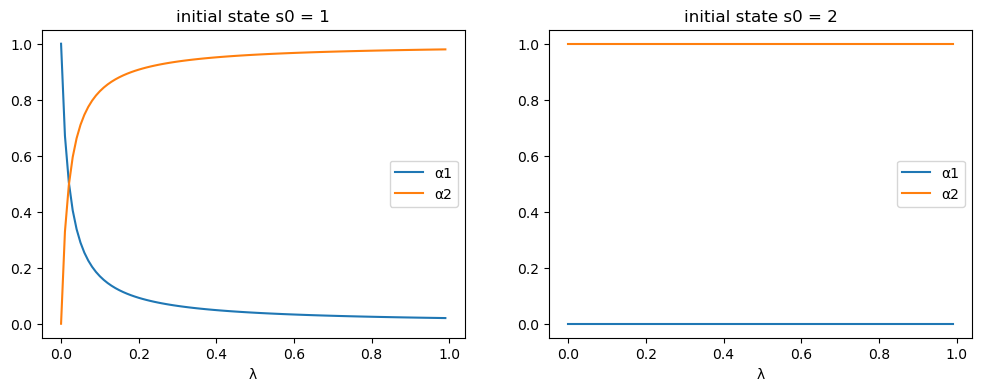
Fig. 102.1 Wealth distribution under different transition#
102.9.4. Example 4#
# dimensions
K, n = 2, 3

# states
s = jnp.array([1, 2, 3])

# transition
λ = .9
μ = .9
δ = .05

# prosperous, moderate, and recession states
P = jnp.array([[1-λ, λ, 0], [μ/2, μ, μ/2], [(1-δ)/2, (1-δ)/2, δ]])

# endowments
ys = jnp.empty((n, K))
ys = ys.at[:, 0].set([.25, .75, .2])       # y1
ys = ys.at[:, 1].set([1.25, .25, .2])      # y2
ex4 = compute_rc_model(s, P, ys)
# endowments
print("ys = \n", ex4.ys)

# pricing kernel
print ("Q = \n", ex4.Q)

# Risk free rate R
print("R = ", ex4.R)

# natural debt limit, A = [A1, A2, ..., AI]
print("A = \n", ex4.A)

print('')

for i in range(1, 4):
    # when the initial state is state i
    ex4 = compute_rc_model(s, P, ys, s0_idx=i-1)
    print(f"when the initial state is state {i}")
    print(f'α = {ex4.α}')
    print(f'ψ = \n{ex4.ψ}')
    print(f'J = \n{ex4.J}\n')
ys =
 [[0.25 1.25]
 [0.75 0.25]
 [0.2  0.2 ]]
Q =
 [[0.09800001 1.080225   0.        ]
 [0.360075   0.88199997 0.6972822 ]
 [0.24038316 0.29440805 0.049     ]]
R =  [0.84873426 0.5156348  1.712941  ]
A =
 [[-1.4141307 -0.4585418]
 [-1.4122484 -1.540054 ]
 [-0.5843434 -0.3823659]]
when the initial state is state 1
α = [0.75514036 0.24485956]
ψ =
[[[ 0.00000013  0.        ]
  [-0.8171543   0.8171544 ]
  [-0.14565787  0.14565794]]]
J =
[[[-2.6574192 -1.5132294]
  [-5.1310315 -2.9217925]
  [-2.6564994 -1.5127057]]]
when the initial state is state 2
α = [0.47835496 0.52164507]
ψ =
[[[ 0.5183286  -0.5183286 ]
  [-0.00000007 -0.00000001]
  [ 0.12191314 -0.12191317]]]
J =
[[[-2.1150534 -2.208685 ]
  [-4.083814  -4.2646008]
  [-2.1143215 -2.2079203]]]
when the initial state is state 3
α = [0.6044665 0.3955335]
ψ =
[[[ 0.28216296 -0.28216296]
  [-0.37231946  0.37231946]
  [-0.00000004  0.00000004]]]
J =
[[[-2.3775644 -1.9232593]
  [-4.590679  -3.713492 ]
  [-2.376742  -1.9225937]]]
102.9.5. Finite Horizon Example#
We now revisit the economy defined in example 1, but set the time horizon to be \(T=10\).
# dimensions
K, n = 2, 2

# states
s = jnp.array([0, 1])

# transition
P = jnp.array([[.5, .5], [.5, .5]])

# endowments
ys = jnp.empty((n, K))
ys = ys.at[:, 0].set(1 - s)       # y1
ys = ys.at[:, 1].set(s)           # y2
ex1_finite = compute_rc_model(s, P, ys, T=10)
# (I + Q + Q^2 + ... + Q^T)
ex1_finite.V[-1]
Array([[5.481717, 4.481717],
       [4.481717, 5.481717]], dtype=float32)
# endowments
ex1_finite.ys
Array([[1., 0.],
       [0., 1.]], dtype=float32)
# pricing kernel
ex1_finite.Q
Array([[0.49, 0.49],
       [0.49, 0.49]], dtype=float32)
# Risk free rate R
ex1_finite.R
Array([1.0204082, 1.0204082], dtype=float32)
In the finite time horizon case, ψ and J are returned as sequences.
Components are ordered from \(t=T\) to \(t=0\).
# when the initial state is state 1
print(f'α = {ex1_finite.α}')
print(f'ψ = \n{ex1_finite.ψ}\n')
print(f'J = \n{ex1_finite.J}')
α = [0.55018353 0.44981652]
ψ =
[[[-0.44981647  0.44981652]
  [ 0.55018353 -0.5501835 ]]

 [[-0.40063658  0.40063673]
  [ 0.59936345 -0.59936327]]

 [[-0.35244036  0.35244054]
  [ 0.64755964 -0.6475595 ]]

 [[-0.30520797  0.3052082 ]
  [ 0.69479203 -0.6947918 ]]

 [[-0.2589203   0.25892067]
  [ 0.7410798  -0.74107945]]

 [[-0.21355844  0.2135588 ]
  [ 0.7864418  -0.78644145]]

 [[-0.16910362  0.16910398]
  [ 0.8308965  -0.83089614]]

 [[-0.12553787  0.12553847]
  [ 0.874462   -0.87446153]]

 [[-0.08284354  0.08284402]
  [ 0.91715634 -0.917156  ]]

 [[-0.04100347  0.04100394]
  [ 0.95899665 -0.9589962 ]]

 [[ 0.00000024  0.00000024]
  [ 1.0000002  -0.99999976]]]

J =
[[[ 1.4834871  1.3413672]
  [ 1.4834871  1.3413672]]

 [[ 2.9373045  2.6559072]
  [ 2.9373045  2.6559072]]

 [[ 4.362046   3.9441566]
  [ 4.362046   3.9441566]]

 [[ 5.758292   5.2066407]
  [ 5.758292   5.2066407]]

 [[ 7.1266136  6.4438753]
  [ 7.1266136  6.4438753]]

 [[ 8.467568   7.6563654]
  [ 8.467568   7.6563654]]

 [[ 9.781704   8.8446045]
  [ 9.781704   8.8446045]]

 [[11.069557  10.009081 ]
  [11.069557  10.009081 ]]

 [[12.331654  11.150267 ]
  [12.331654  11.150267 ]]

 [[13.568508  12.268629 ]
  [13.568508  12.268629 ]]

 [[14.780625  13.364622 ]
  [14.780625  13.364622 ]]]
# when the initial state is state 2
ex1_finite = compute_rc_model(s, P, ys, s0_idx=1, T=10)
print(f'α = {ex1_finite.α}')
print(f'ψ = \n{ex1_finite.ψ}\n')
print(f'J = \n{ex1_finite.J}')
α = [0.44981652 0.55018353]
ψ =
[[[-0.5501835   0.55018353]
  [ 0.44981652 -0.44981647]]

 [[-0.59936327  0.59936345]
  [ 0.40063673 -0.40063658]]

 [[-0.6475595   0.64755964]
  [ 0.35244054 -0.35244036]]

 [[-0.6947918   0.69479203]
  [ 0.3052082  -0.30520797]]

 [[-0.74107945  0.7410798 ]
  [ 0.25892067 -0.2589203 ]]

 [[-0.78644145  0.7864418 ]
  [ 0.2135588  -0.21355844]]

 [[-0.83089614  0.8308965 ]
  [ 0.16910398 -0.16910362]]

 [[-0.87446153  0.874462  ]
  [ 0.12553847 -0.12553787]]

 [[-0.917156    0.91715634]
  [ 0.08284402 -0.08284354]]

 [[-0.9589962   0.95899665]
  [ 0.04100394 -0.04100347]]

 [[-0.99999976  1.0000002 ]
  [ 0.00000024  0.00000024]]]

J =
[[[ 1.3413672  1.4834871]
  [ 1.3413672  1.4834871]]

 [[ 2.6559072  2.9373045]
  [ 2.6559072  2.9373045]]

 [[ 3.9441566  4.362046 ]
  [ 3.9441566  4.362046 ]]

 [[ 5.2066407  5.758292 ]
  [ 5.2066407  5.758292 ]]

 [[ 6.4438753  7.1266136]
  [ 6.4438753  7.1266136]]

 [[ 7.6563654  8.467568 ]
  [ 7.6563654  8.467568 ]]

 [[ 8.8446045  9.781704 ]
  [ 8.8446045  9.781704 ]]

 [[10.009081  11.069557 ]
  [10.009081  11.069557 ]]

 [[11.150267  12.331654 ]
  [11.150267  12.331654 ]]

 [[12.268629  13.568508 ]
  [12.268629  13.568508 ]]

 [[13.364622  14.780625 ]
  [13.364622  14.780625 ]]]
We can check the results with finite horizon converges to the ones with infinite horizon as \(T \rightarrow \infty\).
ex1_large = compute_rc_model(s, P, ys, s0_idx=1, T=10000)
ex1_large.α
Array([0.48999998, 0.51 ], dtype=float32)
ex1.V, ex1_large.V[-1]
(Array([[[25.500013, 24.500013],
         [24.500013, 25.500013]]], dtype=float32),
 Array([[25.500002, 24.500002],
        [24.500002, 25.500002]], dtype=float32))
ex1.ψ, ex1_large.ψ[-1]
(Array([[[-0.99999905,  1.        ],
         [ 0.00000095,  0.        ]]], dtype=float32),
 Array([[-1.0000006 ,  0.9999999 ],
        [-0.00000042, -0.00000034]], dtype=float32))
ex1.J, ex1_large.J[-1]
(Array([[[70.000046, 71.41432 ],
         [70.000046, 71.41432 ]]], dtype=float32),
 Array([[69.99999 , 71.41428 ],
        [69.99999 , 71.414276]], dtype=float32))